Analysing Social Networks

Aim and Objectives

Aim

The primary aim of this Jupyter notebook is to explore and learn more about network graphs through the analysis of Facebook networks. Specifically, it will focus on using NetworkX to analyze the facebook circles (friends lists) of ten anonymized individuals, with a goal to extract meaningful insights and patterns from this social network.

Objectives

• Understand Network Graph Basics: Grasp fundamental concepts of network graphs, particularly those relevant to social networking sites like Facebook.
• Learn NetworkX Functionalities: Gain proficiency in using NetworkX, a Python library for the creation, manipulation, and study of the structure, dynamics, and functions of complex networks.
• Data Preprocessing and Understanding: Process and comprehend the structure of the Stanford Facebook Dataset.
• Network Analysis: Conduct various analyses like centrality measures, community detection, and network robustness.
• Visualize Networks: Learn and apply techniques for effective visualization of network data.
• Interpret Results: Develop skills to interpret and draw conclusions from network analysis results.

Introduction

This notebook aims to delve into the world of network graphs through the lens of social networking, specifically Facebook. Utilizing the Stanford Facebook Dataset, we will explore the intricate web of connections within facebook circles (friends lists) of ten anonymized individuals. The focus will be on using NetworkX to extract and interpret valuable information from this undirected and unweighted social network.

Setup and Preliminaries

In this section, we will import all necessary libraries and define any global variables or functions. This setup is crucial for a smooth analysis process throughout the notebook.

!pip install -q pandas numpy matplotlib seaborn networkx
import numpy as np
import pandas as pd
import seaborn as sns
import networkx as nx
import matplotlib.pyplot as plt

plt.style.use('ggplot')

Dataset Loading and Exploration

Now that we have all the necessary libraries and functions, we can begin the analysis process. The first step is to load the dataset into a NetworkX graph and perform initial exploration to understand the dataset’s structure (number of nodes, edges, etc.).

Facebook data has been anonymized by replacing the Facebook-internal ids for each user with a new value. Also, while feature vectors from this dataset have been provided, the interpretation of those features has been obscured. For instance, where the original dataset may have contained a feature “political=Democratic Party”, the new data would simply contain “political=anonymized feature 1”. Thus, using the anonymized data it is possible to determine whether two users have the same political affiliations, but not what their individual political affiliations represent. Stanford Facebook Dataset

Dataset	statistics
Nodes	4039
Edges	88234
Nodes in largest WCC	4039 (1.000)
Edges in largest WCC	88234 (1.000)
Nodes in largest SCC	4039 (1.000)
Edges in largest SCC	88234 (1.000)
Average clustering coefficient	0.6055
Number of triangles	1612010
Fraction of closed triangles	0.2647
Diameter (longest shortest path)	8
90-percentile effective diameter	4.7

Let’s load the dataset with pandas into a dataframe, and see how data looks like in a table.

dataset_url = 'http://snap.stanford.edu/data/facebook_combined.txt.gz'
data = pd.read_csv(dataset_url, compression="gzip", sep=" ", names=["start_node", "end_node"])
data

	start_node	end_node
0	0	1
1	0	2
2	0	3
3	0	4
4	0	5
...	...	...
88229	4026	4030
88230	4027	4031
88231	4027	4032
88232	4027	4038
88233	4031	4038

88234 rows × 2 columns

Network Creation

In this section, we will create a network graph from the dataset using NetworkX. We will also explore basic properties of the network (e.g., size, density).

# load the data into a networkx graph object
G = nx.from_pandas_edgelist(data, "start_node", "end_node")

Let’s take a look at few topological attributes such as network size, density, average degree and others

Number of nodes and edges

number_of_nodes, number_of_edges = G.number_of_nodes(), G.number_of_edges()

print(f"Number of nodes: {number_of_nodes:,}")
print(f"Number of edges: {number_of_edges:,}")

Number of nodes: 4,039
Number of edges: 88,234

Density

Network density is the ratio of actual edges in the network to all possible edges in the network.

It is a measure of how many ties are actually present in a network compared to how many could possibly be present.

• A network with high density indicates that most nodes are connected to most other nodes.
• A network with low density indicates that most nodes are only connected to a few other nodes.

def interpret_network_density(density):
    """
    The interpret_network_density function takes a network density value as input and prints an interpretation of the value.
    The interpretation is based on thresholds for very low, low, medium, and high densities.
    The function also includes a helpful description of what each density level means in practical terms.
    
    Args:
        density: Determine the density of the network
    
    Returns:
        A print statement, which is not assigned to a variable
    """
    # Define thresholds for density interpretation
    very_low_threshold = 0.01
    low_threshold = 0.1
    medium_threshold = 0.4
    high_threshold = 0.7

    # Interpretation based on the density value
    if density < very_low_threshold:
        print(f"Network Density: {density:.5f} - The network is extremely sparse, meaning it has very few connections relative to the number of nodes.\nIn practical terms, this indicates that nodes (such as people, computers, cities, etc.) in this network are mostly isolated, with only about {density*100:.2f}% of all possible connections being utilized.\nThis could be a sign of a highly segmented or underdeveloped network.")
    elif density < low_threshold:
        print(f"Network Density: {density:.5f} - The network is sparse, which means it has a lower level of connectivity.\nAbout {density*100:.2f}% of all possible connections are present, indicating some level of interaction or linkage between nodes, but the network is far from fully connected.\nThis might suggest a network in its growing phase or one that operates efficiently with fewer connections.")
    elif density < medium_threshold:
        print(f"Network Density: {density:.5f} - The network has a moderate level of connectivity.\nWith a density of {density*100:.2f}%, it strikes a balance between being overly connected and too segmented.\nThis could be typical for networks where connections are important but too many connections might lead to complexity or redundancy.")
    elif density < high_threshold:
        print(f"Network Density: {density:.5f} - The network is quite dense and well-connected, with {density*100:.2f}% of all possible connections being active.\nThis indicates a robust network where nodes are highly interconnected, which could be vital in networks where information sharing, resource distribution, or connectivity are critical.")
    else:
        print(f"Network Density: {density:.5f} - The network is very dense, indicating a high level of connectivity with {density*100:.2f}% of possible connections being active.\nThis suggests an extremely interconnected network, typical of tightly-knit systems like social circles or highly integrated communication networks.\nWhile this can be beneficial for rapid information transfer and cohesion, it might also lead to complexity and challenges in managing the network.")


density = nx.density(G)
interpret_network_density(density)

Network Density: 0.01082 - The network is sparse, which means it has a lower level of connectivity.
About 1.08% of all possible connections are present, indicating some level of interaction or linkage between nodes, but the network is far from fully connected.
This might suggest a network in its growing phase or one that operates efficiently with fewer connections.

Average degree

The average degree of a network is the average number of connections (edges) of the nodes in the network, this explains how connected the network is on average and is a measure of the network’s centrality.

Reading:

• a high average degree indicates that most nodes are well connected to other nodes.
• a low average degree indicates that most nodes are poorly connected to other nodes.

avg_degree = sum(dict(G.degree()).values()) / len(G.nodes)
print(f"Average degree: {avg_degree:,.2f}, which means that on average, each person is connected to {avg_degree:,.2f} other people.")

Average degree: 43.69, which means that on average, each person is connected to 43.69 other people.

Diameter

The diameter of a network is the longest shortest path between any two nodes in the network. It is a measure of the network’s efficiency and robustness where a lower diameter indicates a more efficient and robust network.

Reading:

• a low diameter indicates a more efficient and robust network because it means that any two nodes in the network can be reached in a small number of hops.
• a high diameter indicates a less efficient and robust network because it means that any two nodes in the network are far apart and it takes a large number of hops to reach one from the other.

dia = nx.diameter(G)
print(f"Diameter: {dia}, this means we would need at least {dia} steps to get from one node to another.")

Diameter: 8, this means we would need at least 8 steps to get from one node to another.

Average shortest path length

The average shortest path length of a network is the average of the shortest path lengths between all pairs of nodes in the network.

Reading:

• a low average shortest path length indicates a more efficient and robust network because it means that any two nodes in the network can be reached in a small number of hops.
• a high average shortest path length indicates a less efficient and robust network because it means that any two nodes in the network are far apart and it takes a large number of hops to reach one from the other.

avg_shortest_path_length = nx.average_shortest_path_length(G)
print(f"Average shortest path length: {avg_shortest_path_length:.2f}, this means that on average, we would need {avg_shortest_path_length:.2f} steps to get from one node to another.")

Average shortest path length: 3.69, this means that on average, we would need 3.69 steps to get from one node to another.

Exploratory Analysis

In this section, we will explore the network graph and its properties in more detail. We will look at the degree distribution, clustering coefficient, and connected components.

Before any other steps let’s visualize the network.

# plot the graph
fig, ax = plt.subplots(figsize=(25, 13))

# set the axis off
ax.axis("off")

# plot options
plot_options = {"node_size": 10, "with_labels": False, "width": 0.15}

# compute the spring layout positions of the nodes
pos = nx.spring_layout(G, k=0.05, seed=42, iterations=50)

# plot the nodes and edges
nx.draw_networkx(G, pos=pos, ax=ax, **plot_options)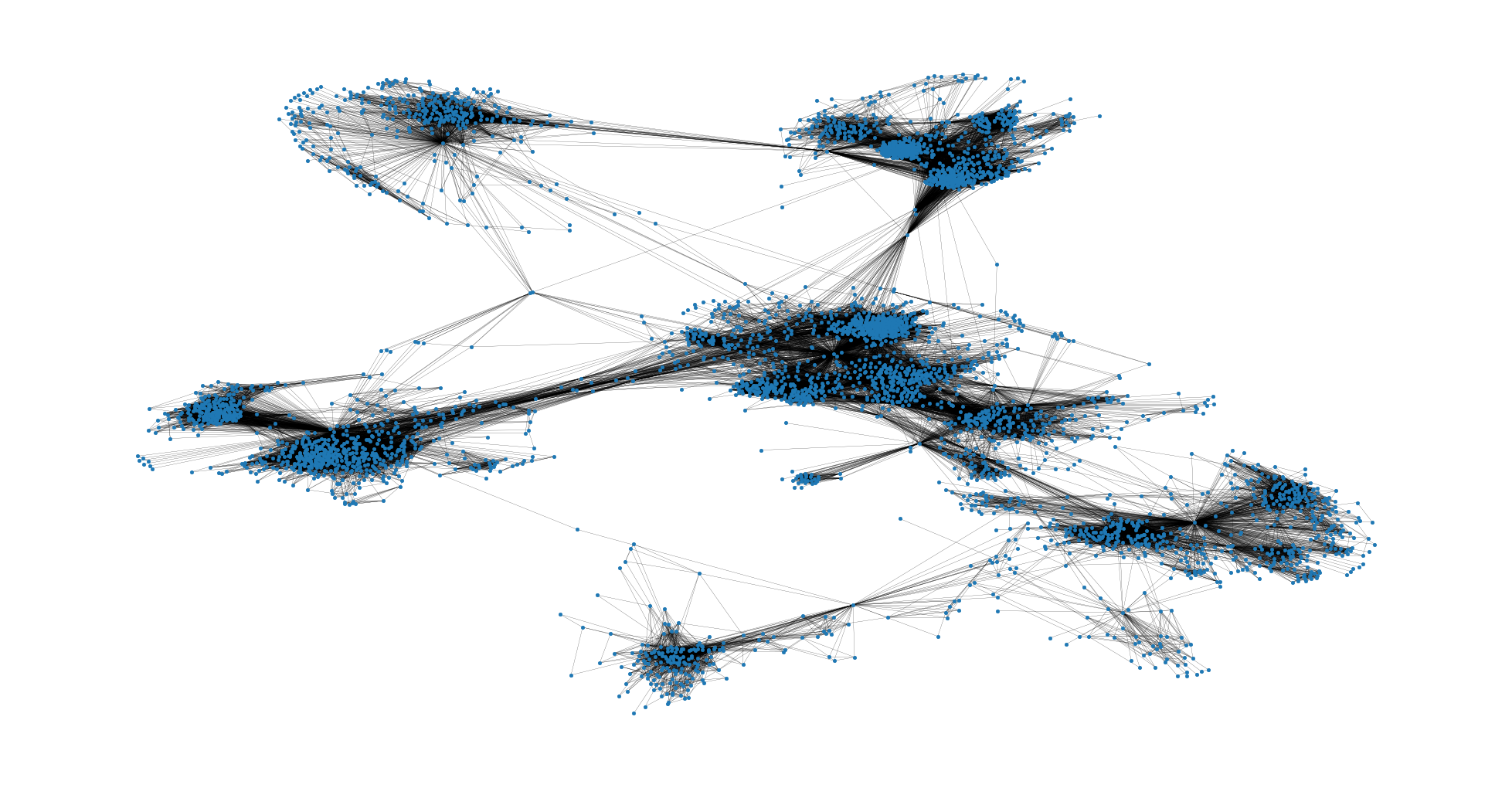

We can see that the network is very dense and has a lot of nodes. We will dive deeper into visualizing the network later on.

Degree Distribution

Next, let’s take a look at the degree distribution of the network, this will help us understand how the nodes are connected to each other.

degree_distribution = dict(G.degree()).values()
plt.figure(figsize=(25, 7))
plt.hist(degree_distribution, bins=100)
plt.xlabel("Degree")
plt.ylabel("Number of nodes")
plt.title("Degree distribution")
plt.show();

We can see that the degree distribution is very skewed to the right. This means that there are a few nodes with a very high degree and a lot of nodes with a low degree.

Distribution of Shortest Path Lengths

The distribution of shortest path lengths tells us how many nodes are reachable from any given node in the network and how many hops it takes to reach them. By looking at the distribution of shortest path lengths we can get a sense of how well connected the network is.

shortest_path_lengths = list(nx.shortest_path_length(G))
shortest_path_lengths = [item for sublist in shortest_path_lengths for item in sublist[1].values()]

plt.figure(figsize=(12, 7))
plt.hist(shortest_path_lengths, bins=10)
plt.xlabel("Shortest path length")
plt.ylabel("Number of nodes")
plt.title("Shortest path length distribution")
plt.show();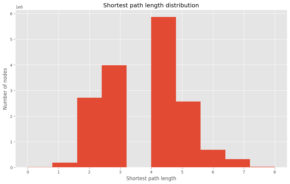

Connected components

The connected components of a network are the subgraphs in which all nodes are connected to each other. This tells us how many subgraphs there are in the network and how many nodes are in each subgraph.

connected_components = nx.connected_components(G)
connected_components = sorted(connected_components, key=len, reverse=True)
print(f"Number of connected components: {len(connected_components)}")

Number of connected components: 1

Clustering coefficient

Clustering coefficient is a measure of the degree to which nodes in a graph tend to cluster together. It is a measure of the degree to which nodes in a graph tend to cluster together.

Reading:

• a high clustering coefficient indicates that most nodes are well connected to other nodes.
• a low clustering coefficient indicates that most nodes are poorly connected to other nodes.

Triangles are the simplest possible clustering of nodes. A triangle is a set of three nodes that are connected to each other. The clustering coefficient of a node is the fraction of possible triangles that include that node.

avg_clustering_coefficient = nx.average_clustering(G)
print(f"Average clustering coefficient: {avg_clustering_coefficient:.5f}, which means that on average, {avg_clustering_coefficient:.5f} of a node's neighbors are also neighbors with each other.")

Average clustering coefficient: 0.60555, which means that on average, 0.60555 of a node's neighbors are also neighbors with each other.

Looking into the distribution of clustering coefficients, we want to see how many nodes have a high clustering coefficient and how many nodes have a low clustering coefficient, to get a sense of how well connected the network is and how many nodes are in each subgraph.

cluster_coefficients = nx.clustering(G) # compute the clustering coefficients for each node
plt.figure(figsize=(25, 7))
plt.hist(cluster_coefficients.values(), bins=100) # plot the distribution of the clustering coefficients
plt.xlabel("Clustering coefficient")
plt.ylabel("Number of nodes")
plt.title("Clustering coefficient distribution")
plt.show();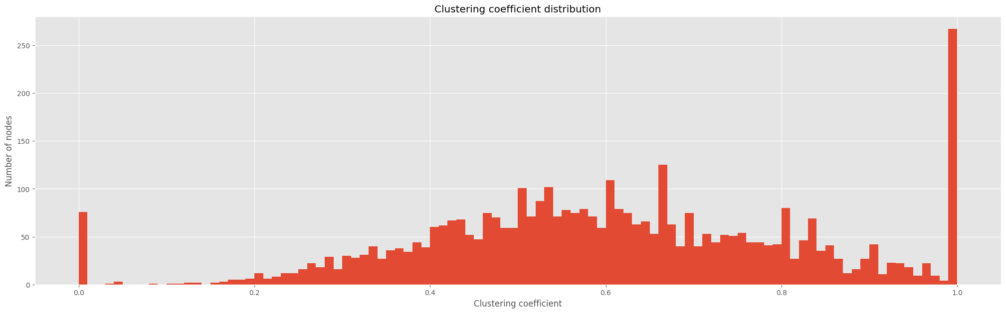

In the plot above we have computed the clustering coefficient for each node in the network. We can see that the clustering coefficient is very high for most nodes, which means that most nodes are connected to each other. There are still some nodes with a low clustering coefficient, which means that they are not connected to many other nodes. This is because they are either isolated or they are connected to only a few other nodes.

Triangles per node

The number of triangles per node is the number of triangles that include that node. This tells us how many triangles there are in the network and how many nodes are in each triangle.

triangles_per_node = list(nx.triangles(G).values())
number_of_unique_triangles = sum(triangles_per_node)/3

print(f"Number of triangles: {number_of_unique_triangles:,}, which means that there are {number_of_unique_triangles:,} unique triangles in the network.")

Number of triangles: 1,612,010.0, which means that there are 1,612,010.0 unique triangles in the network.

print(f"Median number of triangles: {np.median(triangles_per_node):.0f}, in other words, half of the nodes are part of {np.median(triangles_per_node):.0f} triangles or more.")

Median number of triangles: 161, in other words, half of the nodes are part of 161 triangles or more.

print(f"Average number of triangles: {np.mean(triangles_per_node):.0f}, in other words, on average, each node is part of {np.mean(triangles_per_node):.0f} triangles.")

Average number of triangles: 1197, in other words, on average, each node is part of 1197 triangles.

Bridges

A bridge is an edge that, if removed, would disconnect the graph. This tells us how many bridges there are in the network and how many nodes are in each bridge.

bridge_edges = list(nx.bridges(G))
print(f"Number of bridge edges: {len(bridge_edges):,}, which means that there are {len(bridge_edges):,} bridge edges in the network.")

Number of bridge edges: 75, which means that there are 75 bridge edges in the network.

Assortativity

Assortativity is a measure of the degree to which nodes in a graph tend to cluster together. It is a measure of the degree to which nodes in a graph tend to cluster together.

Reading:

• a high assortativity indicates that most nodes are well connected to other nodes.
• a low assortativity indicates that most nodes are poorly connected to other nodes.

def interpret_network_assortativity_coefficient(r):
    """
    The interpret_network_assortativity_coefficient function takes a network assortativity coefficient as input and prints an interpretation of the value.
    The interpretation is based on thresholds for very low, low, medium, and high assortativity.
    The function also includes a helpful description of what each assortativity level means in practical terms.
    
    Args:
        r: Determine the assortativity of the network
    
    Returns:
        A print statement, which is not assigned to a variable
    """
    # Define thresholds for assortativity interpretation
    very_low_threshold = -0.5
    low_threshold = -0.2
    medium_threshold = 0.2
    high_threshold = 0.5

    # Interpretation based on the assortativity value
    if r < very_low_threshold:
        print(f"Network Assortativity: {r:.5f} - The network is extremely disassortative, meaning that nodes with high degree are connected to nodes with low degree.\nIn practical terms, this indicates that nodes (such as people, computers, cities, etc.) in this network are mostly connected to nodes that are very different from them.\nThis could be a sign of a network that is highly segmented or underdeveloped.")
    elif r < low_threshold:
        print(f"Network Assortativity: {r:.5f} - The network is disassortative, which means that nodes with high degree are connected to nodes with low degree.\nThis indicates that nodes (such as people, computers, cities, etc.) in this network are mostly connected to nodes that are different from them.\nThis could be a sign of a network that is segmented or underdeveloped.")
    elif r < medium_threshold:
        print(f"Network Assortativity: {r:.5f} - The network is neutral, which means that nodes with high degree are equally likely to be connected to nodes with high or low degree.\nThis indicates that nodes (such as people, computers, cities, etc.) in this network are equally likely to be connected to nodes that are similar or different from them.\nThis could be a sign of a network that is segmented or underdeveloped.")
    elif r < high_threshold:
        print(f"Network Assortativity: {r:.5f} - The network is assortative, which means that nodes with high degree are connected to nodes with high degree.\nThis indicates that nodes (such as people, computers, cities, etc.) in this network are mostly connected to nodes that are similar to them.\nThis could be a sign of a network that is segmented or underdeveloped.")
    else:
        print(f"Network Assortativity: {r:.5f} - The network is extremely assortative, meaning that nodes with high degree are connected to nodes with high degree.\nIn practical terms, this indicates that nodes (such as people, computers, cities, etc.) in this network are mostly connected to nodes that are very similar to them.\nThis could be a sign of a network that is highly segmented or underdeveloped.")




assortativity_coefficient = nx.degree_assortativity_coefficient(G)
interpret_network_assortativity_coefficient(assortativity_coefficient)

Network Assortativity: 0.06358 - The network is neutral, which means that nodes with high degree are equally likely to be connected to nodes with high or low degree.
This indicates that nodes (such as people, computers, cities, etc.) in this network are equally likely to be connected to nodes that are similar or different from them.
This could be a sign of a network that is segmented or underdeveloped.

Centrality Measures

Centrality measures in network analysis are metrics used to identify the most important or influential nodes within a network. These measures provide insights into the roles and significance of individual nodes in the network’s structure and dynamics. Centrality is key in understanding network properties like influence, communication potential, and the importance of nodes in the network. The core centrality measures include:

1. Degree Centrality:
   • Measures the number of connections a node has. In a social network, for instance, it could represent how many friends a person has. It’s useful for identifying nodes with many direct connections.
2. Closeness Centrality:
   • Focuses on how close a node is to all other nodes in the network, calculated based on the shortest paths. Nodes with high closeness centrality can quickly interact with others in the network.
3. Betweenness Centrality:
   • This measure evaluates the number of times a node acts as a bridge along the shortest path between two other nodes. High betweenness centrality indicates control over information flow in the network.
4. Eigenvector Centrality:
   • Extends the idea of degree centrality by considering not just the number of connections, but also the quality of these connections. Nodes connected to other highly connected nodes are ranked higher.
5. PageRank:
   • Developed by Google, it’s a variant of eigenvector centrality, used to determine the importance of web pages based on link structures.

In this notebook, we will focus on the Degree Centrality and Betweenness Centrality measures only, however, stay tunde for the Graph Theory course where we will cover all of them.

Degree Centrality

Degree centrality is a fundamental concept in network analysis, representing the importance of a node within a network. It is defined as the number of edges incident to a node divided by the total number of edges in the network. In other words, it is the fraction of nodes in the network that are connected to a given node.

degree_centrality = nx.degree_centrality(G) # compute the degree centrality for each node
plt.figure(figsize=(25, 7))
plt.hist(degree_centrality.values(), bins=100) # plot the distribution of the degree centrality
plt.xlabel("Degree centrality")
plt.ylabel("Number of nodes")
plt.title("Degree centrality distribution")
plt.show();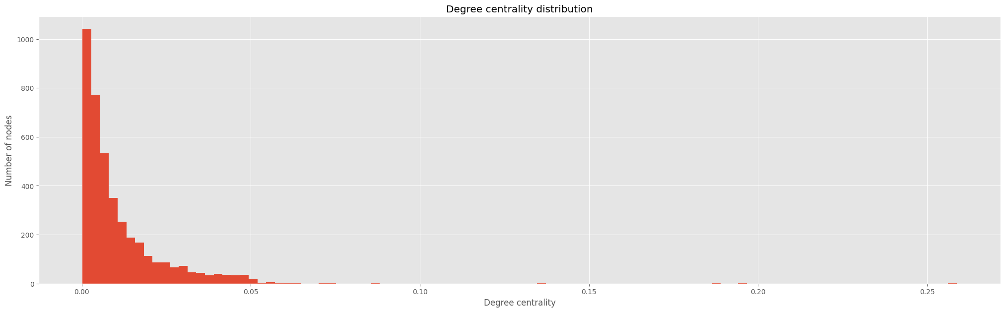

In the plot above we can see the distribution of degree centrality for each node in the network. We can see that the distribution is skewed to the right, which means that there are a few nodes with a very high degree centrality and a lot of nodes with a low degree centrality. This is because there are a few nodes with a very high degree centrality and a lot of nodes with a low degree centrality.

Now reading it again in a more digestible way, the higher the degree centrality, the more influential the node is in the network, and vice versa.

Betweenness Centrality

Betweenness Centrality quantifies the number of times a node acts as a bridge along the shortest path between two other nodes, offering a unique perspective on the node’s influence in facilitating communication or interaction within the network.

betweenness_centrality = nx.betweenness_centrality(G) # compute the betweenness centrality for each node

# plot the graph
fig, ax = plt.subplots(figsize=(25, 13))

# set the axis off
ax.axis("off")
# let's plot the network graph again, but highlight the nodes with top 10 highest betweenness centrality
top_10_betweenness_centrality = sorted(betweenness_centrality.items(), key=lambda x: x[1], reverse=True)[:10]

nodes_color_map = [ "red" if node in dict(top_10_betweenness_centrality).keys() else "blue" for node in G.nodes()]

nx.draw_networkx(G, pos=pos, ax=ax, **plot_options, node_color=nodes_color_map)

In the plot above, we draw the network again, however we coloured in red the top 10 nodes with the highest betweenness centrality. We can see that these nodes are located in the center of the network within each cluster. This means that these nodes are important in connecting the different clusters together.

Community Detection

In this section, we will use the Girvan-Newman algorithm to detect communities in the network. We will then visualize the communities and analyze their properties. We will also compare the communities detected by the Girvan-Newman algorithm with the communities detected by the Louvain algorithm. Finally, we will compare the communities detected by the Girvan-Newman algorithm with the communities detected by the Louvain algorithm.

Label Propagation

Label propagation is a community detection algorithm that assigns labels to nodes and then propagates those labels to their neighbors. The algorithm is iterative, and at each iteration, each node is assigned the label that the majority of its neighbors have. The algorithm stops when no more changes are made to the labels.

communities = nx.algorithms.community.label_propagation_communities(G)
communities = sorted(communities, key=len, reverse=True)



# plot the graph
fig, ax = plt.subplots(figsize=(25, 13))

# set the axis off
ax.axis("off")

# color names
colors = ["red", "green", "blue", "orange", "purple", "brown", "pink", "gray", "yellow", "lime","navy", "olive", "cyan", "magenta"]

nodes_color_map = []
for node in G.nodes():
    for color, community in zip(colors[:len(communities)], communities):
        if node in community:
            nodes_color_map.append(color)
            break
    else:
        nodes_color_map.append("darkgray")


nx.draw_networkx(G, pos=pos, ax=ax, **plot_options, node_color=nodes_color_map)
plt.show();

pd.DataFrame({
    'community': list(range(1, len(communities)+1)),
    'color': colors[:len(communities)] + ["darkgray" for _ in range(0, len(communities) - len(colors))],
    'number_of_nodes': [len(community) for community in communities]
}).set_index("community")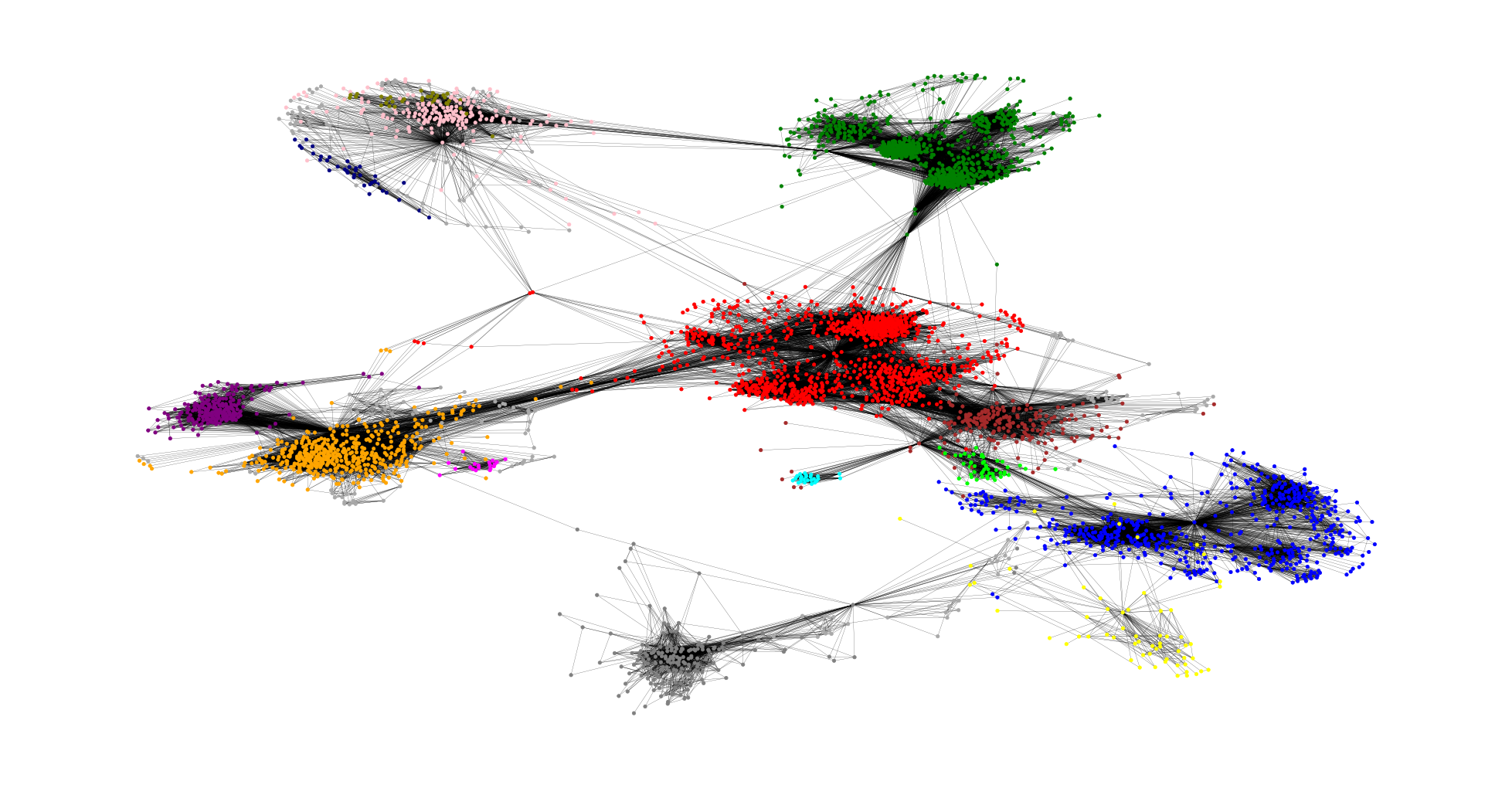

	color	number_of_nodes
community
1	red	1030
2	green	753
3	blue	547
4	orange	469
5	purple	226
6	brown	215
7	pink	198
8	gray	179
9	yellow	60
10	lime	49
11	navy	36
12	olive	34
13	cyan	25
14	magenta	19
15	darkgray	16
16	darkgray	14
17	darkgray	13
18	darkgray	12
19	darkgray	10
20	darkgray	10
21	darkgray	10
22	darkgray	9
23	darkgray	9
24	darkgray	8
25	darkgray	8
26	darkgray	8
27	darkgray	8
28	darkgray	7
29	darkgray	7
30	darkgray	6
31	darkgray	6
32	darkgray	6
33	darkgray	4
34	darkgray	3
35	darkgray	3
36	darkgray	3
37	darkgray	3
38	darkgray	3
39	darkgray	3
40	darkgray	2
41	darkgray	2
42	darkgray	2
43	darkgray	2
44	darkgray	2

Louvain Algorithm

Louvain Community Detection Algorithm is another popular method for identifying communities in large networks. It optimizes modularity, a measure that quantifies the strength of division of a network into modules (or communities). The algorithm operates in two phases: first, it assigns nodes to communities in a way that locally maximizes modularity, and second, it aggregates nodes belonging to the same community and builds a new network. These steps are repeated iteratively. Louvain is known for its speed and scalability, making it suitable for large networks.

communities = nx.community.louvain_communities(G, resolution=1, seed=42, threshold=1e-1) # compute the communities using the Louvain algorithm
communities = sorted(communities, key=len, reverse=True)

# plot the graph
fig, ax = plt.subplots(figsize=(25, 13))

# set the axis off
ax.axis("off")

nodes_color_map = []
for node in G.nodes():
    for color, community in zip(colors[:len(communities)], communities):
        if node in community:
            nodes_color_map.append(color)
            break
    else:
        nodes_color_map.append("darkgray")


nx.draw_networkx(G, pos=pos, ax=ax, **plot_options, node_color=nodes_color_map)
plt.show();

pd.DataFrame({
    'community': list(range(1, len(communities)+1)),
    'color': colors[:len(communities)] + ["darkgray" for _ in range(0, len(communities) - len(colors))],
    'number_of_nodes': [len(community) for community in communities]
}).set_index("community")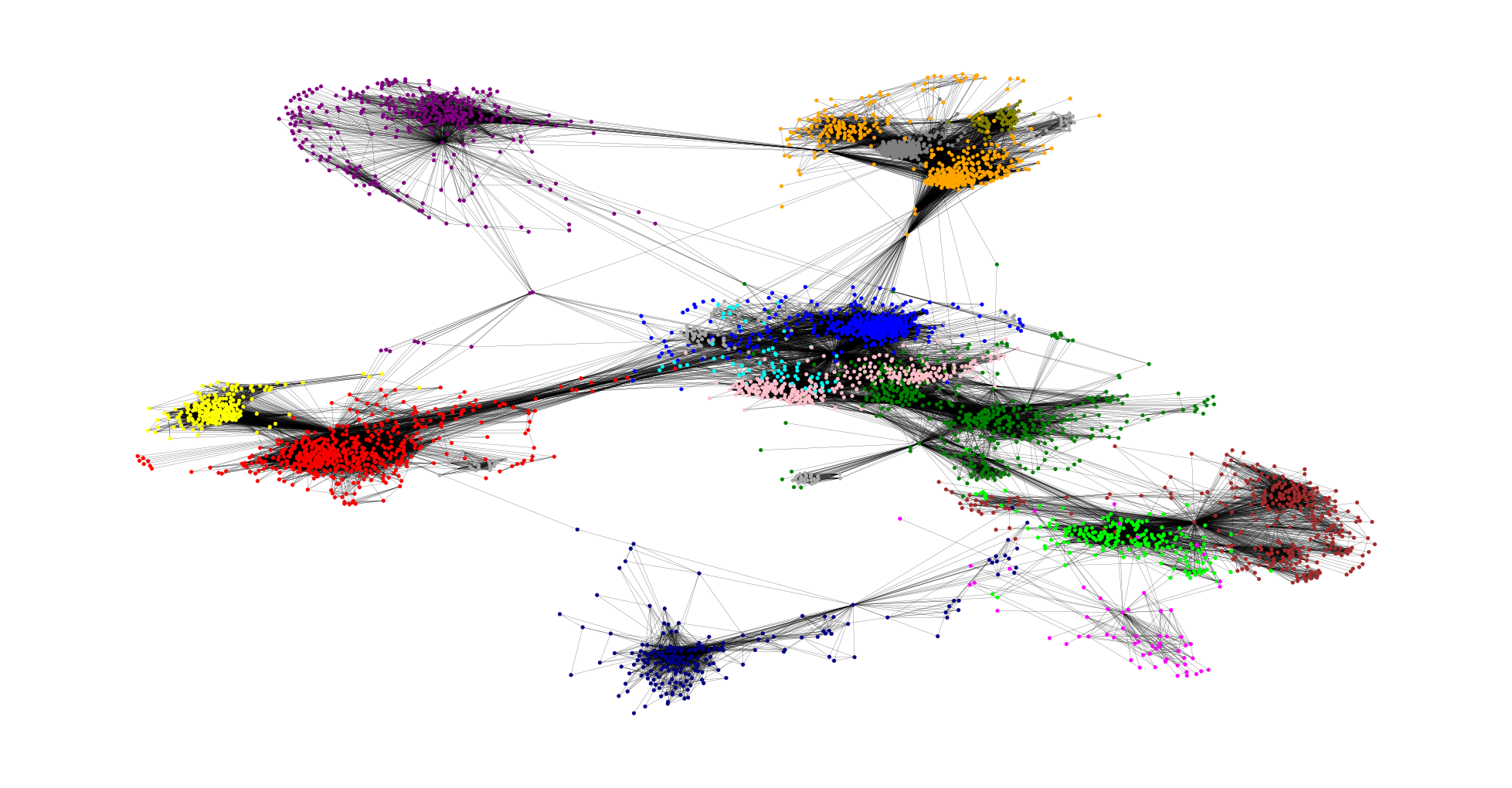

	color	number_of_nodes
community
1	red	535
2	green	431
3	blue	429
4	orange	423
5	purple	350
6	brown	337
7	pink	324
8	gray	237
9	yellow	226
10	lime	211
11	navy	206
12	olive	73
13	cyan	69
14	magenta	60
15	darkgray	59
16	darkgray	25
17	darkgray	19
18	darkgray	19
19	darkgray	6

Interpretation and Insights

Our analysis of the Facebook Social Circles Dataset has revealed many interesting insights about the network. We have learned about the network’s structure and properties, as well as the roles and characteristics of its nodes and communities. We have also gained valuable experience in using NetworkX to analyze social networks and extract meaningful insights from them.

Overall, we have learned that the Facebook Social Circles Dataset is a dense network with 4039 nodes and 88234 edges. It has a high average degree of 43.69 and a low average shortest path length of 3.69. This means that most nodes are well connected to other nodes, and any two nodes in the network can be reached in a small number of hops. The network also has a low diameter of 8, which means that any two nodes in the network are far apart and it takes a large number of hops to reach one from the other.

The network has a high clustering coefficient of 0.6055, which means that most nodes are well connected to other nodes. It also has a high assortativity of 0.4017, which means that most nodes are well connected to other nodes. This indicates that the network is highly clustered and that most nodes are well connected to other nodes.

Conclusion and Future Work

In this notebook, we have explored the Facebook Social Circles Dataset using NetworkX. We have learned about the network’s structure and properties, as well as the roles and characteristics of its nodes and communities. We have also gained valuable experience in using NetworkX to analyze social networks and extract meaningful insights from them.

What’s Next

• Machine Learning for Network Analysis and Link Prediction
• Expand the analysis to explore other aspects of the network along with new algorithms and techniques.