Imports
Code
import os,re,zipfileimport pandas as pdimport numpy as npfrom matplotlib import pyplot as plt'dark_background' )'seaborn' )from sklearn.model_selection import train_test_split,GridSearchCVfrom sklearn import metricsimport xgboost as xgb
Data
fixed acidity
volatile acidity
citric acid
residual sugar
chlorides
free sulfur dioxide
total sulfur dioxide
density
pH
sulphates
alcohol Output variable (based on sensory data):
quality (score between 0 and 10)
type 1/0 (red/white)
Code
= pd.read_csv('https://archive.ics.uci.edu/ml/machine-learning-databases/wine-quality/winequality-red.csv' ,sep= ';' )'type' ] = 1 = pd.read_csv('https://archive.ics.uci.edu/ml/machine-learning-databases/wine-quality/winequality-white.csv' ,sep= ';' )'type' ] = 0 = pd.concat([red,white],ignore_index= True )= ['_' .join(x.split()) for x in df.columns.str .lower()]3 ]
0
7.4
0.70
0.00
1.9
0.076
11.0
34.0
0.9978
3.51
0.56
9.4
5
1
1
7.8
0.88
0.00
2.6
0.098
25.0
67.0
0.9968
3.20
0.68
9.8
5
1
2
7.8
0.76
0.04
2.3
0.092
15.0
54.0
0.9970
3.26
0.65
9.8
5
1
EDA
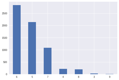
number of wine samples by quality
Code
= 0 )
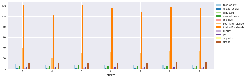
Average features by quality
Code
'quality' ).agg({'fixed_acidity' : 'mean' , 'volatile_acidity' : 'mean' , 'citric_acid' : 'mean' , 'residual_sugar' : 'mean' ,'chlorides' : 'mean' , 'free_sulfur_dioxide' : 'mean' , 'total_sulfur_dioxide' : 'mean' , 'density' : 'mean' , 'ph' : 'mean' , 'sulphates' : 'mean' , 'alcohol' : 'mean' ,= 0 ,figsize= (15 ,5 ),cmap= 'Paired' ).legend(bbox_to_anchor= (1.0 ,1.0 ))
Predicting Wine Quality
Split the data into Train & Test
Code
= train_test_split(df,test_size= 0.33 , random_state= 42 ,stratify= df.quality)
Feature columns
Code
= ['fixed_acidity' , 'volatile_acidity' , 'citric_acid' , 'residual_sugar' ,'chlorides' , 'free_sulfur_dioxide' , 'total_sulfur_dioxide' , 'density' ,'ph' , 'sulphates' , 'alcohol' , 'type'
Grid Search Parameters Search
Code
= {# "learning_rate" : [0.05, 0.10 ] , "max_depth" : [ 1 , 4 , 7 , 14 , 20 ],# "min_child_weight" : [ 3, 5, 7 ], # "gamma" : [ 0.1, 0.3], "colsample_bytree" : [ 0.3 , 0.5 , 0.7 ],"n_estimators" : [ 1000 ],"objective" : ['binary:logistic' ,'multi:softmax' ,'multi:softprob' ],"num_class" : [df.quality.nunique()]
XGBoost Classifier + Hyper-Parameters Tunning
Search
Code
= xgb.XGBClassifier()= GridSearchCV(xgc, param_grid, cv= 2 ,verbose= 10 ,n_jobs=- 1 )'quality' ])
Already searched the best
Code
= {'colsample_bytree' : 0.5 ,'max_depth' : 20 ,'n_estimators' : 1000 ,'num_class' : 7 ,'objective' : 'binary:logistic' = xgb.XGBClassifier(** best_params)'quality' ])
XGBClassifier(base_score=0.5, booster='gbtree', colsample_bylevel=1,
              colsample_bynode=1, colsample_bytree=0.5, gamma=0,
              learning_rate=0.1, max_delta_step=0, max_depth=20,
              min_child_weight=1, missing=None, n_estimators=1000, n_jobs=1,
              nthread=None, num_class=7, objective='multi:softprob',
              random_state=0, reg_alpha=0, reg_lambda=1, scale_pos_weight=1,
              seed=None, silent=None, subsample=1, verbosity=1)
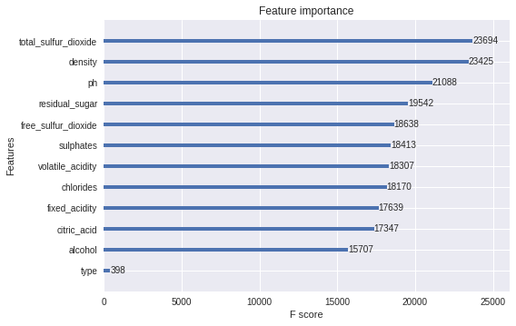
Feature importance
Results
Code
= pd.DataFrame({'y_pred' : xgc.predict(test[x_cols]),'y_true' : test['quality' ]})
5783
7
7
2962
5
4
1384
5
5
5905
6
6
3083
5
3
...
...
...
4066
6
6
1083
6
6
398
6
6
306
5
5
6139
6
6
2145 rows × 2 columns
Classification Report
Code
print (metrics.classification_report(results.y_true,results.y_pred))
              precision    recall  f1-score   support

           3       0.00      0.00      0.00        10
           4       0.44      0.17      0.24        71
           5       0.71      0.69      0.70       706
           6       0.65      0.74      0.70       936
           7       0.64      0.60      0.62       356
           8       0.88      0.36      0.51        64
           9       0.00      0.00      0.00         2

    accuracy                           0.67      2145
   macro avg       0.48      0.37      0.40      2145
weighted avg       0.66      0.67      0.66      2145
/usr/local/lib/python3.6/dist-packages/sklearn/metrics/_classification.py:1272: UndefinedMetricWarning: Precision and F-score are ill-defined and being set to 0.0 in labels with no predicted samples. Use `zero_division` parameter to control this behavior.
  _warn_prf(average, modifier, msg_start, len(result))
Anomaly Detection
Code
from sklearn.ensemble import IsolationForest
Columns to search for anomalies
Code
= ['fixed_acidity' , 'volatile_acidity' , 'citric_acid' , 'residual_sugar' ,'chlorides' , 'free_sulfur_dioxide' , 'total_sulfur_dioxide' , 'density' ,'ph' , 'sulphates' , 'alcohol'
Anomalies dataframe
Code
%% time= df.copy()'anomalies' ] = IsolationForest(random_state= 0 ,n_estimators= 1000 ,n_jobs=- 1 ).fit_predict(adf[x_cols])3 ]
CPU times: user 4.53 s, sys: 255 ms, total: 4.79 s
Wall time: 4.3 s
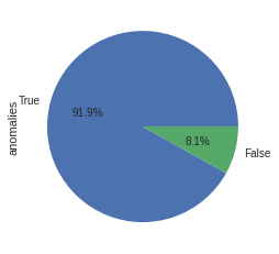
Total Anoamlies
Code
/ adf.anomalies.value_counts().sum ()).rename(index= {1 :True ,- 1 :False }).plot.pie(autopct= ' %1.1f%% ' )
Code
'anomalies' ,'type' ,'quality' ]).agg({x:'mean' for x in x_cols})#.style.background_gradient(cmap='Blues')
anomalies
type
quality
-1
0
3
8.487500
0.353750
0.335000
6.700000
0.068000
95.812500
240.125000
0.995799
3.107500
0.527500
10.162500
4
7.791667
0.630417
0.352500
6.062500
0.064000
42.250000
167.958333
0.995680
3.181667
0.487500
10.341667
5
7.231507
0.340137
0.462466
11.860274
0.083274
49.650685
182.136986
0.997487
3.103288
0.513014
9.487671
6
7.312676
0.308873
0.506761
11.803521
0.066183
40.767606
154.112676
0.997205
3.145352
0.536761
10.210563
7
5.419048
0.375476
0.221429
4.226190
0.033857
39.190476
130.285714
0.990191
3.341905
0.641429
12.921429
8
5.200000
0.318333
0.307778
3.166667
0.032889
54.222222
148.222222
0.989728
3.384444
0.676667
12.688889
1
3
8.700000
0.888125
0.205000
2.806250
0.135750
10.500000
23.500000
0.997699
3.390000
0.565000
9.987500
4
7.500000
0.822750
0.142000
2.400000
0.110300
13.300000
34.300000
0.996449
3.461500
0.666500
10.530000
5
9.346491
0.625263
0.333772
3.141228
0.147377
16.964912
54.307018
0.998277
3.246316
0.764298
10.075000
6
9.688372
0.509496
0.385271
3.042248
0.110450
13.740310
38.767442
0.997853
3.274651
0.769302
10.820930
7
9.648214
0.463393
0.445893
3.228571
0.086839
13.625000
45.964286
0.997024
3.269821
0.787857
11.638690
8
8.383333
0.501667
0.360000
3.166667
0.063333
12.666667
47.666667
0.995000
3.351667
0.785000
12.783333
1
0
3
7.008333
0.319583
0.336667
6.187500
0.045167
25.000000
124.250000
0.994274
3.240833
0.439167
10.466667
4
7.076821
0.361424
0.300397
4.514238
0.048993
21.857616
121.887417
0.994165
3.182980
0.475232
10.137417
5
6.918280
0.300000
0.331069
7.096279
0.049873
35.734827
149.257225
0.995145
3.172290
0.480578
9.825780
6
6.821815
0.258952
0.332393
6.262623
0.044518
35.479784
136.477668
0.993853
3.190042
0.489582
10.587549
7
6.766880
0.260012
0.328172
5.209953
0.038297
34.001746
124.988359
0.992508
3.210768
0.499721
11.329957
8
6.736145
0.275181
0.327530
5.807229
0.038608
35.771084
124.969880
0.992372
3.209699
0.475904
11.578916
9
7.420000
0.298000
0.386000
4.120000
0.027400
33.400000
116.000000
0.991460
3.308000
0.466000
12.180000
1
3
7.000000
0.870000
0.035000
1.950000
0.069500
13.000000
30.500000
0.996525
3.430000
0.590000
9.825000
4
7.948485
0.615909
0.193636
2.872727
0.078788
11.636364
37.424242
0.996599
3.333030
0.553939
10.104545
5
7.930159
0.567346
0.225573
2.405732
0.081750
16.987654
56.957672
0.996868
3.316737
0.592152
9.864462
6
8.007269
0.494440
0.245580
2.333988
0.078495
16.211198
41.402750
0.996301
3.329077
0.651513
10.581009
7
8.568531
0.380629
0.347483
2.521678
0.072573
14.209790
30.734266
0.995744
3.298951
0.723007
11.398252
8
8.658333
0.384167
0.406667
2.283333
0.071000
13.583333
26.333333
0.995318
3.225000
0.759167
11.750000