Using this notebook to learn PyTorch and its applications
Machine Learning
PyTorch
Deep Learning
Author
Daniel Fat
Published
February 3, 2020
What is PyTorch ?
It’s a Python-based scientific computing package targeted at two sets of audiences: * a replacement for NumPy to use the power of GPUs * a deep learning research platform that provides maximum flexibility and speed
From NumPy to PyTorch
Tensors
Tensors are similar to NumPy’s ndarrays, with the addition being that Tensors can also be used on a GPU to accelerate computing.
NumPy to Torch
np.array() == torch.Tensor()
np.ones() == torch.ones()
np.random.rand() == torch.rand()
type(array) == tensor.type
np.shape(array) == tensor.shape
np.resize(array,size) == tensor.view(size)
np.add(x,y) == torch.add(x,y)
np.sub(x,y) == torch.sub(x,y)
np.multiply(x,y) == torch.mul(x,y)
np.divide(x,y) == torch.div(x,y)
np.mean(array) == tensor.mean()
np.std(array) == tensor.std()
We can also convert arrays NumPy <-> PyTorch
Variables
A Variable wraps a Tensor. It supports nearly all the API’s defined by a Tensor. Variable also provides a backward method to perform backpropagation.
For example, to backpropagate a loss function to train model parameter x, we use a variable loss to store the value computed by a loss function.
Then, we call loss.backward which computes the gradients for all trainable parameters.
PyTorch will store the gradient results back in the corresponding variable x.
Autograd is a PyTorch package for the differentiation for all operations on Tensors. It performs the backpropagation starting from a variable.
In deep learning, this variable often holds the value of the cost function. backward executes the backward pass and computes all the backpropagation gradients automatically.
import torchimport pandas as pdimport numpy as npimport os,re,sys,iofrom matplotlib import pyplot as pltfrom sklearn.datasets import load_bostonfrom sklearn.model_selection import train_test_splitfrom sklearn.preprocessing import MinMaxScalerfrom sklearn import metricsfrom time import timeimport seaborn as snsscaler = MinMaxScaler()plt.style.use('seaborn')
/usr/local/lib/python3.6/dist-packages/statsmodels/tools/_testing.py:19: FutureWarning: pandas.util.testing is deprecated. Use the functions in the public API at pandas.testing instead.
  import pandas.util.testing as tm
Linear Regression
Boston Dataset
The Boston house-price data of Harrison, D. and Rubinfeld, D.L. ‘Hedonic prices and the demand for clean air’, J. Environ. Economics & Management, vol.5, 81-102, 1978. Used in Belsley, Kuh & Welsch, ‘Regression diagnostics …’, Wiley, 1980. N.B. Various transformations are used in the table on pages 244-261 of the latter.
CRIM per capita crime rate by town
ZN proportion of residential land zoned for lots over 25,000 sq.ft.
INDUS proportion of non-retail business acres per town
CHAS Charles River dummy variable (= 1 if tract bounds river; 0 otherwise)
NOX nitric oxides concentration (parts per 10 million)
RM average number of rooms per dwelling
AGE proportion of owner-occupied units built prior to 1940
DIS weighted distances to five Boston employment centres
RAD index of accessibility to radial highways
TAX full-value property-tax rate per $10,000
PTRATIO pupil-teacher ratio by town
B 1000(Bk - 0.63)^2 where Bk is the proportion of blacks by town
LSTAT % lower status of the population
MEDV Median value of owner-occupied homes in $1000 s
It can be seen that the value range of data is different and the difference is large, so we need to make standardization.
Suppose each feature has a mean value μ and a standard deviation σ on the whole dataset. Hence we can subtract each value of the feature and then divide μ by σ to get the normalized value of each feature. (Tutorial approach)
Another option is to use the MinMaxScaler from sklearn
Code
# apply the min max scaling for each column but not PRICEfor col in boston.columns[:-1]: boston[[col]] = scaler.fit_transform(boston[[col]])
PyTorch Linear Rregression
Then we split the data into train/test while casting the data to numpy arrays
At the heart of PyTorch data loading utility is the torch.utils.data.DataLoader class. It represents a Python iterable over a dataset, with support for
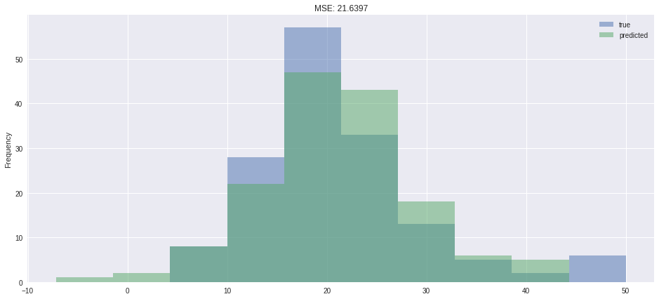
We can compare the predictions with the actual targets, using the following method:
Calculate the difference between the two matrices (preds and targets). Square all elements of the difference matrix to remove negative values. Calculate the average of the elements in the resulting matrix. The result is a single number, known as the mean squared error (MSE).
Code
loss = torch.nn.MSELoss()
Optimizers
Rather than manually updating the weights of the model as we have been doing, we use the optim package to define an Optimizer that will update the weights for us.
pred = pd.DataFrame({'true': [x[0].tolist() for x in y_test],'predicted': [x[0].tolist() for x in net(X_test)],})pred.plot.hist(alpha=0.5,figsize=(16,7),title=f'MSE: {loss(net(X_test), y_test).item():.4f}')
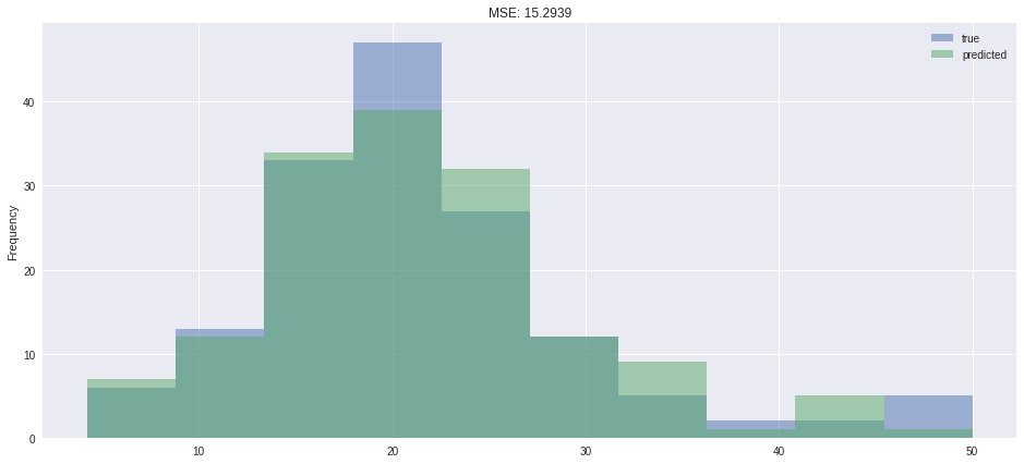
pred = pd.DataFrame({'true': [x[0] for x in y_test.tolist()],'predicted': glm_gaussian.predict(X_test)})pred.plot.hist(alpha=0.5,figsize=(16,7),title=f"MSE: {metrics.mean_squared_error(pred['true'],pred.predicted):.4f}")
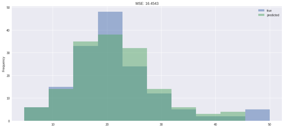
pred = pd.DataFrame({'true': [x[0] for x in y_test.tolist()],'predicted': glm_gamma.predict(X_test)})pred.plot.hist(alpha=0.5,figsize=(16,7),title=f"MSE: {metrics.mean_squared_error(pred['true'],pred.predicted):.4f}")
The MNIST database (Modified National Institute of Standards and Technology database) is a large database of handwritten digits that is commonly used for training various image processing systems
Code
from torchvision import datasets, transforms
Compose a transformer to nomralize the data
transforms.ToTensor() converts the image into numbers, that are understandable by the system. It separates the image into three color channels (separate images): red, green & blue. Then it converts the pixels of each image to the brightness of their color between 0 and 255. These values are then scaled down to a range between 0 and 1.
transforms.Normalize() normalizes the tensor with a mean and standard deviation which goes as the two parameters respectively.
Code
# Define a transform to normalize the datatransform = transforms.Compose([transforms.ToTensor(), transforms.Normalize((0.5,), (0.5,)), ])
Download the dataset and normalize it
Code
# Download and load the training datatrainset = datasets.MNIST('drive/My Drive/mnist/MNIST_data/', download=True, train=True, transform=transform)valset = datasets.MNIST('drive/My Drive/mnist/MNIST_data/', download=True, train=False, transform=transform)
Then we define a Seqeuntial model with 3 levels of layers, Linear which applies a linear transformation and ReLu which applies the rectified linear, the output of this chain of transofrmation being passed into LogSoftmax activation function
Code
# Layer details for the neural networkinput_size =784hidden_sizes = [128, 64]output_size =10# Build a feed-forward networkmodel = torch.nn.Sequential(torch.nn.Linear(input_size, hidden_sizes[0]), torch.nn.ReLU(), torch.nn.Linear(hidden_sizes[0], hidden_sizes[1]), torch.nn.ReLU(), torch.nn.Linear(hidden_sizes[1], output_size), torch.nn.LogSoftmax(dim=1))print(model)
This time on the training process we reshape each image matrix into one 1x1 array
Code
time0 = time()epochs =15for e inrange(epochs): running_loss =0for images, labels in trainloader:# Flatten MNIST images into a 784 long vector images = images.view(images.shape[0], -1) optimizer.zero_grad() output = model(images) l = loss(output, labels) l.backward() optimizer.step() running_loss += l.item()else:print("Epoch {} - Training loss: {}".format(e, running_loss/len(trainloader)))print("\nTraining Time (in minutes) =",(time()-time0)/60)
Epoch 0 - Training loss: 0.6175047809492423
Epoch 1 - Training loss: 0.27926216799535475
Epoch 2 - Training loss: 0.21707710018877918
Epoch 3 - Training loss: 0.17828493828434488
Epoch 4 - Training loss: 0.14850337554349194
Epoch 5 - Training loss: 0.12661053494476815
Epoch 6 - Training loss: 0.11251892998659693
Epoch 7 - Training loss: 0.10000329123718589
Epoch 8 - Training loss: 0.08876785766164552
Epoch 9 - Training loss: 0.08140811096054754
Epoch 10 - Training loss: 0.07434628869015683
Epoch 11 - Training loss: 0.06872579670681962
Epoch 12 - Training loss: 0.06227882651151466
Epoch 13 - Training loss: 0.05694495400846767
Epoch 14 - Training loss: 0.05275964385930147

Training Time (in minutes) = 3.717697087923686
Validation Process
Code
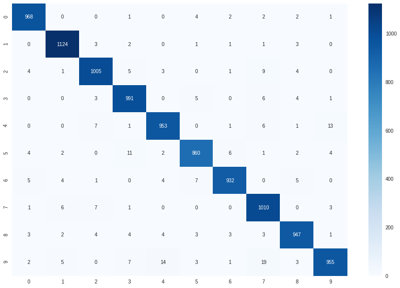
y_true,y_pred =list(),list()correct_count, all_count =0, 0for images,labels in valloader:for i inrange(len(labels)): img = images[i].view(1, 784)# Turn off gradients to speed up this partwith torch.no_grad(): logps = model(img)# Output of the network are log-probabilities, need to take exponential for probabilities ps = torch.exp(logps) probab =list(ps.numpy()[0]) pred_label = probab.index(max(probab)) true_label = labels.numpy()[i] y_true.append(true_label) y_pred.append(pred_label)if(true_label == pred_label): correct_count +=1 all_count +=1print("Number Of Images Tested =", all_count)print("\nModel Accuracy =", (correct_count/all_count))
Number Of Images Tested = 10000

Model Accuracy = 0.9745
X_train = np.array([x.flatten() for x in trainset.data.numpy()])y_train = np.array([x.flatten() for x in trainset.targets.numpy()])X_test = np.array([x.flatten() for x in valset.data.numpy()])y_test = np.array([x.flatten() for x in valset.targets.numpy()])
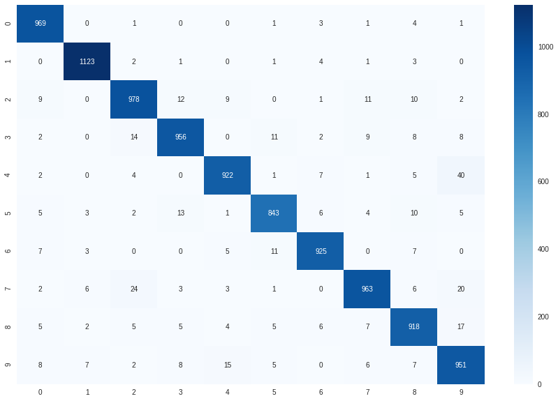
For the XGBClassifier the multi:softmax objective is used to permit training on multiple label classificaiton