Imports
Code
import pandas as pdimport numpy as npfrom sklearn import preprocessingimport matplotlib.pyplot as pltimport seaborn as snsfrom sklearn import metricsfrom sklearn.model_selection import train_test_split from keras.layers import Input, Densefrom keras.models import Model, Sequentialfrom keras import regularizersimport xgboost as xgb'seaborn' )
Data
The datasets contains transactions made by credit cards in September 2013 by european cardholders. This dataset presents transactions that occurred in two days, where we have 492 frauds out of 284,807 transactions. The dataset is highly unbalanced, the positive class (frauds) account for 0.172% of all transactions.
It contains only numerical input variables which are the result of a PCA transformation. Unfortunately, due to confidentiality issues, we cannot provide the original features and more background information about the data. Features V1, V2, … V28 are the principal components obtained with PCA, the only features which have not been transformed with PCA are ‘Time’ and ‘Amount’. Feature ‘Time’ contains the seconds elapsed between each transaction and the first transaction in the dataset. The feature ‘Amount’ is the transaction Amount, this feature can be used for example-dependant cost-senstive learning. Feature ‘Class’ is the response variable and it takes value 1 in case of fraud and 0 otherwise.
Code
= pd.read_csv('data/creditcard.csv' )
0
0.0
-1.359807
-0.072781
2.536347
1.378155
-0.338321
0.462388
0.239599
0.098698
0.363787
...
-0.018307
0.277838
-0.110474
0.066928
0.128539
-0.189115
0.133558
-0.021053
149.62
0
1
0.0
1.191857
0.266151
0.166480
0.448154
0.060018
-0.082361
-0.078803
0.085102
-0.255425
...
-0.225775
-0.638672
0.101288
-0.339846
0.167170
0.125895
-0.008983
0.014724
2.69
0
2
1.0
-1.358354
-1.340163
1.773209
0.379780
-0.503198
1.800499
0.791461
0.247676
-1.514654
...
0.247998
0.771679
0.909412
-0.689281
-0.327642
-0.139097
-0.055353
-0.059752
378.66
0
3
1.0
-0.966272
-0.185226
1.792993
-0.863291
-0.010309
1.247203
0.237609
0.377436
-1.387024
...
-0.108300
0.005274
-0.190321
-1.175575
0.647376
-0.221929
0.062723
0.061458
123.50
0
4
2.0
-1.158233
0.877737
1.548718
0.403034
-0.407193
0.095921
0.592941
-0.270533
0.817739
...
-0.009431
0.798278
-0.137458
0.141267
-0.206010
0.502292
0.219422
0.215153
69.99
0
...
...
...
...
...
...
...
...
...
...
...
...
...
...
...
...
...
...
...
...
...
...
284802
172786.0
-11.881118
10.071785
-9.834783
-2.066656
-5.364473
-2.606837
-4.918215
7.305334
1.914428
...
0.213454
0.111864
1.014480
-0.509348
1.436807
0.250034
0.943651
0.823731
0.77
0
284803
172787.0
-0.732789
-0.055080
2.035030
-0.738589
0.868229
1.058415
0.024330
0.294869
0.584800
...
0.214205
0.924384
0.012463
-1.016226
-0.606624
-0.395255
0.068472
-0.053527
24.79
0
284804
172788.0
1.919565
-0.301254
-3.249640
-0.557828
2.630515
3.031260
-0.296827
0.708417
0.432454
...
0.232045
0.578229
-0.037501
0.640134
0.265745
-0.087371
0.004455
-0.026561
67.88
0
284805
172788.0
-0.240440
0.530483
0.702510
0.689799
-0.377961
0.623708
-0.686180
0.679145
0.392087
...
0.265245
0.800049
-0.163298
0.123205
-0.569159
0.546668
0.108821
0.104533
10.00
0
284806
172792.0
-0.533413
-0.189733
0.703337
-0.506271
-0.012546
-0.649617
1.577006
-0.414650
0.486180
...
0.261057
0.643078
0.376777
0.008797
-0.473649
-0.818267
-0.002415
0.013649
217.00
0
284807 rows × 31 columns
EDA
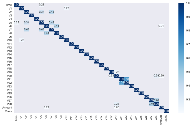
Feature Correlation
Code
= df.corr(method= 'spearman' )= (12 ,7 ))> .2 ],annot= True ,fmt= '.2f' ,cmap= 'Blues' );
Modeling
Select Features for modeling
Code
= ['Time' ,'V1' ,'V2' ,'V3' ,'V4' ,'V5' ,'V6' ,'V7' ,'V8' ,'V9' ,'V10' ,'V11' ,'V12' ,'V13' ,'V14' ,'V15' ,'V16' ,'V17' ,'V18' ,'V19' ,'V20' ,'V21' ,'V22' ,'V23' ,'V24' ,'V25' ,'V26' ,'V27' ,'V28' ,'Amount' ]= 'Class'
Train Test Split
Code
= train_test_split(df, test_size= 0.33 ,random_state= 42 ,stratify= df[target])
Autoencoder
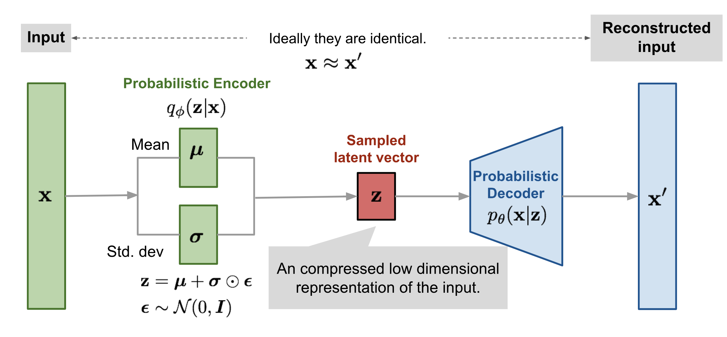
Autoencoder is a neural network designed to learn an identity function in an unsupervised way to reconstruct the original input while compressing the data in the process so as to discover a more efficient and compressed representation.
The encoder network essentially accomplishes the dimensionality reduction, just like how we would use Principal Component Analysis (PCA) or Matrix Factorization (MF) for. In addition, the autoencoder is explicitly optimized for the data reconstruction from the code. A good intermediate representation not only can capture latent variables, but also benefits a full decompression process.
Define a generalistic Auto Encoder
Code
def autoencoder(shape,regularizer= regularizers.l1(10e-5 )):## input layer X_train.shape[1] = Input(shape= (shape,))## encoding part = Dense(100 , activation= 'tanh' , activity_regularizer= regularizer)(input_layer)= Dense(50 , activation= 'relu' )(encoded)## decoding part = Dense(50 , activation= 'tanh' )(encoded)= Dense(100 , activation= 'tanh' )(decoded)## output layer = Dense(shape, activation= 'relu' )(decoded)= Model(input_layer, output_layer)compile (optimizer= "adadelta" , loss= "mse" )return autoencoder
Pass the shape of your X_train
Code
= autoencoder(train[features].shape[1 ])
Keras model Summary
Code
Model: "model"
_________________________________________________________________
Layer (type)                 Output Shape              Param #
=================================================================
input_1 (InputLayer)         [(None, 30)]              0
_________________________________________________________________
dense (Dense)                (None, 100)               3100
_________________________________________________________________
dense_1 (Dense)              (None, 50)                5050
_________________________________________________________________
dense_2 (Dense)              (None, 50)                2550
_________________________________________________________________
dense_3 (Dense)              (None, 100)               5100
_________________________________________________________________
dense_4 (Dense)              (None, 30)                3030
=================================================================
Total params: 18,830
Trainable params: 18,830
Non-trainable params: 0
_________________________________________________________________
Let’s normalize our data
Code
= preprocessing.MinMaxScaler().fit(train[features].values)
Code
= df.copy()= scaler.transform(df[features])= scaled_data.loc[scaled_data[target] == 1 ],scaled_data.loc[scaled_data[target] == 0 ]
Now we can fit our Autoencoder
Code
= 20 , shuffle = True , validation_split = 0.25 )
Epoch 1/20
6676/6676 [==============================] - 9s 1ms/step - loss: 0.1457 - val_loss: 0.0821
Epoch 2/20
6676/6676 [==============================] - 6s 845us/step - loss: 0.0772 - val_loss: 0.0821
Epoch 3/20
6676/6676 [==============================] - 6s 867us/step - loss: 0.0770 - val_loss: 0.0818
Epoch 4/20
6676/6676 [==============================] - 5s 790us/step - loss: 0.0769 - val_loss: 0.0814
Epoch 5/20
6676/6676 [==============================] - 7s 976us/step - loss: 0.0768 - val_loss: 0.0810
Epoch 6/20
6676/6676 [==============================] - 5s 783us/step - loss: 0.0712 - val_loss: 0.0603
Epoch 7/20
6676/6676 [==============================] - 5s 722us/step - loss: 0.0559 - val_loss: 0.0599
Epoch 8/20
6676/6676 [==============================] - 5s 717us/step - loss: 0.0558 - val_loss: 0.0596
Epoch 9/20
6676/6676 [==============================] - 5s 713us/step - loss: 0.0557 - val_loss: 0.0593
Epoch 10/20
6676/6676 [==============================] - 5s 710us/step - loss: 0.0556 - val_loss: 0.0590
Epoch 11/20
6676/6676 [==============================] - 5s 801us/step - loss: 0.0555 - val_loss: 0.0586
Epoch 12/20
6676/6676 [==============================] - 5s 768us/step - loss: 0.0554 - val_loss: 0.0584
Epoch 13/20
6676/6676 [==============================] - 5s 748us/step - loss: 0.0553 - val_loss: 0.0581
Epoch 14/20
6676/6676 [==============================] - 8s 1ms/step - loss: 0.0552 - val_loss: 0.0577
Epoch 15/20
6676/6676 [==============================] - 6s 835us/step - loss: 0.0551 - val_loss: 0.0575
Epoch 16/20
6676/6676 [==============================] - 6s 862us/step - loss: 0.0550 - val_loss: 0.0572
Epoch 17/20
6676/6676 [==============================] - 7s 1ms/step - loss: 0.0549 - val_loss: 0.0569
Epoch 18/20
6676/6676 [==============================] - 6s 971us/step - loss: 0.0548 - val_loss: 0.0409
Epoch 19/20
6676/6676 [==============================] - 6s 957us/step - loss: 0.0261 - val_loss: 0.0248
Epoch 20/20
6676/6676 [==============================] - 6s 855us/step - loss: 0.0229 - val_loss: 0.0245
<tensorflow.python.keras.callbacks.History at 0x7fee661db190>
We extract the hidden layers so then our model can encode given data
Code
= Sequential()0 ])1 ])2 ])
then we encode the two dataframes that contains fraudulent and non fraudulent samples
Code
= hidden_representation.predict(fraud[features])= hidden_representation.predict(non_fraud[features])
finally we ca bring them back together into a dataframe where we can see that we have a higher number of features than the initial one, this being a result of our 3rd layer which has an output shape of 50
Code
= pd.DataFrame(np.append(fraud_hidden, non_fraud_hidden, axis = 0 ))= np.append(np.ones(fraud_hidden.shape[0 ]), np.zeros(non_fraud_hidden.shape[0 ]))= encoded_df[target].astype(int )3 ]
0
0.0
0.176606
0.482658
0.149698
0.0
0.0
0.675127
0.0
0.677855
0.018553
...
0.257808
0.0
0.070143
0.015373
0.0
0.0
0.0
0.0
0.153822
1
1
0.0
0.141019
0.480566
0.048828
0.0
0.0
0.617751
0.0
0.668253
0.000000
...
0.260265
0.0
0.094272
0.000000
0.0
0.0
0.0
0.0
0.217649
1
2
0.0
0.151974
0.425213
0.094413
0.0
0.0
0.695415
0.0
0.605650
0.000000
...
0.183696
0.0
0.106665
0.000000
0.0
0.0
0.0
0.0
0.159188
1
3 rows × 51 columns
Classification models
Now that we have encoded data we wan to train an XGBoost model to classify fraudulent accounts.
We will use first the raw data to train the classifier, then in the second part we will use the encoded data.
Before Autoencoding
train the classifier
Code
%% time= xgb.XGBClassifier(objective= 'binary:logistic' ,use_label_encoder= False ,eval_metric= 'logloss' )
CPU times: user 2min 49s, sys: 896 ms, total: 2min 50s
Wall time: 23.3 s
XGBClassifier(base_score=0.5, booster='gbtree', colsample_bylevel=1,
              colsample_bynode=1, colsample_bytree=1, eval_metric='logloss',
              gamma=0, gpu_id=-1, importance_type='gain',
              interaction_constraints='', learning_rate=0.300000012,
              max_delta_step=0, max_depth=6, min_child_weight=1, missing=nan,
              monotone_constraints='()', n_estimators=100, n_jobs=8,
              num_parallel_tree=1, objective='binary:logistic', random_state=0,
              reg_alpha=0, reg_lambda=1, scale_pos_weight=1, subsample=1,
              tree_method='exact', use_label_encoder=False,
              validate_parameters=1, verbosity=None)
make predictions on the test data
Code
= test.copy()'y_pred' ] = clf.predict(test[features])
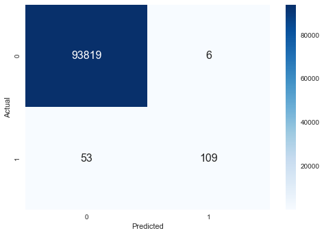
Classification Report
Code
print (metrics.classification_report(test[target],test['y_pred' ]))
              precision    recall  f1-score   support

           0       1.00      1.00      1.00     93825
           1       0.97      0.77      0.86       162

    accuracy                           1.00     93987
   macro avg       0.98      0.89      0.93     93987
weighted avg       1.00      1.00      1.00     93987
Confusion Matrix
Code
'y_pred' ]),cmap= 'Blues' ,annot= True ,fmt= 'd' , annot_kws= {'size' : 16 })'Predicted' )'Actual' );
After Autoencoding
Train test split the encoded data
Code
= train_test_split(encoded_df,test_size= 0.33 ,random_state= 42 ,stratify= encoded_df[target])
train the classifier
Code
%% time= xgb.XGBClassifier(objective= 'binary:logistic' ,use_label_encoder= False ,eval_metric= 'logloss' )= 1 ),encoded_train[target])
CPU times: user 3min 27s, sys: 1.74 s, total: 3min 29s
Wall time: 29.2 s
XGBClassifier(base_score=0.5, booster='gbtree', colsample_bylevel=1,
              colsample_bynode=1, colsample_bytree=1, eval_metric='logloss',
              gamma=0, gpu_id=-1, importance_type='gain',
              interaction_constraints='', learning_rate=0.300000012,
              max_delta_step=0, max_depth=6, min_child_weight=1, missing=nan,
              monotone_constraints='()', n_estimators=100, n_jobs=8,
              num_parallel_tree=1, objective='binary:logistic', random_state=0,
              reg_alpha=0, reg_lambda=1, scale_pos_weight=1, subsample=1,
              tree_method='exact', use_label_encoder=False,
              validate_parameters=1, verbosity=None)
make predictions on the test data
Code
= encoded_test.copy()'y_pred' ] = enc_clf.predict(encoded_test.drop([target],axis= 1 ))
Classification Report
Code
print (metrics.classification_report(encoded_test[target],encoded_test['y_pred' ]))
              precision    recall  f1-score   support

           0       1.00      1.00      1.00     93825
           1       0.95      0.67      0.79       162

    accuracy                           1.00     93987
   macro avg       0.97      0.84      0.89     93987
weighted avg       1.00      1.00      1.00     93987
Confusion Matrix
Code
'y_pred' ]),cmap= 'Blues' ,annot= True ,fmt= 'd' , annot_kws= {'size' : 16 })'Predicted' )'Actual' );
Conclusions
Here we have seen an example usage of the autoencoder architecture
Another aspect we can observe is the contrast between the orignal data vs encoded data through the xgboost model. In the same time the loss value from the autoencoder is playing a big role in the difference between the results from the both classifiers.
The current data in this example is not illustrating the full potention of autoencoders since it has already being processed by PCA
-png.png) .{preview-image}
.{preview-image}