Probability Distributions


Aim: Get familiar with probability distibutions and how they work
Objectives:
- Get Familiar with common probability distributions
- Bernoulli Distribution
- Uniform Distribution
- Binomial Distribution
- Normal Distribution
- Gamma Distribution
- Poisson Distribution
- Exponential Distribution
- Tweedie Distribution
- Highlight the main differences between Tweedie Distribution based model and the traditinal Frequency-Severity models
Imports
import pandas as pd
import numpy as np
import scipy.stats as ss

import matplotlib.pyplot as plt
import seaborn as sns
sns.set_style('whitegrid')
A probability distribution is a list of all of the possible outcomes of a random variable along with their corresponding probability values
$f(k;p) =pk + (1-p)(1-k)$
- $p$ = probability
- $k$ = possible outcomes
- $f$ = probability mass function
A Bernoulli event is one for which the probability the event occurs is p and the probability the event does not occur is $1-p$; i.e., the event is has two possible outcomes (usually viewed as success or failure) occurring with probability $p$ and $1-p$, respectively. A Bernoulli trial is an instantiation of a Bernoulli event. So long as the probability of success or failure remains the same from trial to trial (i.e., each trial is independent of the others), a sequence of Bernoulli trials is called a Bernoulli process. Among other conclusions that could be reached, this means that for n trials, the probability of n successes is $p^n$.
A Bernoulli distribution is the pair of probabilities of a Bernoulli event
random_bernoulli = ss.bernoulli(p=0.5).rvs(size=10)
random_bernoulli.mean()
plt.hist(random_bernoulli,label='Original Population',alpha=.7);
plt.hist(ss.bernoulli(p=random_bernoulli.mean()).rvs(size=10),label='Random Samples with Bernoulli',alpha=.7);
plt.xlabel('Value')
plt.ylabel('Frequency');
plt.legend(bbox_to_anchor=(1, -0.128),ncol=2);

$P(k;n) = \frac{n!}{k!(n-k)!} p^k(1-p)^{(n-k)}$
The binomial distribution is a probability distribution that summarizes the likelihood that a value will take one of two independent values under a given set of parameters or assumptions. The underlying assumptions of the binomial distribution are that there is only one outcome for each trial, that each trial has the same probability of success, and that each trial is mutually exclusive, or independent of each other.
random_binomial = np.random.binomial(1,p=.5,size=10)
random_binomial.mean()
plt.hist(random_binomial,label='Original Population',alpha=.7);
plt.hist(np.random.binomial(1,p=random_binomial.mean(),size=10),label='Random Samples with Binomial',alpha=.7);
plt.xlabel('Value')
plt.ylabel('Frequency');
plt.legend(bbox_to_anchor=(1, -0.128),ncol=2);

The Bernoulli distribution represents the success or failure of a single Bernoulli trial. The Binomial Distribution represents the number of successes and failures in n independent Bernoulli trials for some given value of n. For example, if a manufactured item is defective with probability p, then the binomial distribution represents the number of successes and failures in a lot of n items. In particular, sampling from this distribution gives a count of the number of defective items in a sample lot.
Let's review Probability Mass Function(PMF)
In probability and statistics, a probability mass function (PMF) is a function that gives the probability that a discrete random variable is exactly equal to some value. Sometimes it is also known as the discrete density function.
A probability mass function differs from a probability density function (PDF) in that the latter is associated with continuous rather than discrete random variables. A PDF must be integrated over an interval to yield a probability.
The Poisson distribution describes the probability to find exactly x events in a given length of time if the events occur independently at a constant rate.
In addition, the Poisson distribution can be obtained as an approximation of a binomial distribution when the number of trials $n$ of the latter distribution is large, success probability $p$ is small, and $np$ is a finite number.
The PMF of the Poisson distribution is given by $P(X = x) = \frac{e^{-λ}λ^x}{x!}, x=0,1,...\infty$ where λ is a positive number.
Both the mean and variance of the Poisson distribution are equal to λ.
The maximum likelihood estimate of λ from a sample from the Poisson distribution is the sample mean.
x = np.random.randint(5,100,size=100)
x.mean()
random_poisson = np.random.poisson(x,size=100)
random_poisson.mean()
plt.hist(x,label='Original Population',alpha=.7);
plt.hist(random_poisson,label='Random Samples with Poisson',alpha=.7);
plt.xlabel('Value')
plt.ylabel('Frequency');
plt.legend(bbox_to_anchor=(1, -0.128),ncol=2);

Before this let's review the Probability Density Function(PDF)
We capture the notion of being close to a number with a probability density function which is often denoted by $ρ(x)$
While the absolute likelihood for a continuous random variable to take on any particular value is 0 (since there is an infinite set of possible values to begin with), the value of the PDF at two different samples can be used to infer, in any particular draw of the random variable, how much more likely it is that the random variable would equal one sample compared to the other sample.
The probability density function is $p(x) = \frac{1}{b - a}$
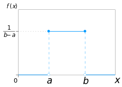
In statistics, a type of probability distribution in which all outcomes are equally likely. A deck of cards has within it uniform distributions because the likelihood of drawing a heart, a club, a diamond or a spade is equally likely. A coin also has a uniform distribution because the probability of getting either heads or tails in a coin toss is the same.
This distribution is defined by two parameters, $a$ and $b$:
- $a$ is the minimum.
- $b$ is the maximum.
low = 5 # min - also known as loc in the context of uniform distribution
high = 10 # max - also know as scale in the context of uniform distribution
random_uniform = np.random.uniform(low,high,size=100)
plt.hist(random_uniform,label='Original Population',alpha=.7);
plt.hist(np.random.uniform(random_uniform.min(),random_uniform.max(),size=100),label='Random Samples with Uniform',alpha=.7);
plt.xlabel('Value')
plt.ylabel('Frequency');
plt.legend(bbox_to_anchor=(1, -0.128),ncol=2);

$f(x)= {\frac{1}{\sigma\sqrt{2\pi}}}e^{- {\frac {1}{2}} (\frac {x-\mu}{\sigma})^2}$
Normal distribution, also known as the Gaussian distribution, is a probability distribution that is symmetric about the mean, showing that data near the mean are more frequent in occurrence than data far from the mean. In graph form, normal distribution will appear as a bell curve.
The normal distribution model is motivated by the Central Limit Theorem. This theory states that averages calculated from independent, identically distributed random variables have approximately normal distributions, regardless of the type of distribution from which the variables are sampled (provided it has finite variance). Normal distribution is sometimes confused with symmetrical distribution.
The normal distribution has two parameters:
- $mu$ - mean
- $sigma$ - standard deviation
random_vals = np.random.randint(1,100,size=10)
random_vals
mu = random_vals.mean()
sigma = random_vals.std()
random_normal = np.random.normal(mu,sigma,size=10)
plt.hist(random_vals,label='Original Population',alpha=.7);
plt.hist(random_normal,label='Random Samples with Normal',alpha=.7);
plt.xlabel('Value')
plt.ylabel('Frequency');
plt.legend(bbox_to_anchor=(1, -0.128),ncol=2);

where $G(a)$ is the Gamma function, and the parameters a and b are both positive, i.e. $a > 0$ and $b$ > 0$
- $a$ (alpha) is known as the shape parameter, while $b$ (beta) is referred to as the scale parameter.
- $b$ has the effect of stretching or compressing the range of the Gamma distribution.
A Gamma distribution with $b = 1$ is known as the standard Gamma distribution.
The Gamma distribution represents a family of shapes. As suggested by its name, a controls the shape of the family of distributions. The fundamental shapes are characterized by the following values of a:
Case I (a < 1)
- When a < 1, the Gamma distribution is exponentially shaped and asymptotic to both the vertical and horizontal axes.
Case II (a = 1)
- A Gamma distribution with shape parameter a = 1 and scale parameter b is the same as an exponential distribution of scale parameter (or mean) b.
Case III (a > 1)
- When a is greater than one, the Gamma distribution assumes a mounded (unimodal), but skewed shape. The skewness reduces as the value of a increases.
The Gamma distribution is sometimes called the Erlang distribution, when its shape parameter a is an integer.
x = np.random.gamma(500,size=100)
m = x.mean()
v = x.var()
m,v
a = m**2/v # calculate alpha parameter - also known as shape
b = m/v # calculate beta parameter - also known as scale
random_gamma = np.random.gamma(a,1/b,size=100)
random_gamma.mean()
plt.hist(x,label='Original Population',alpha=.7);
plt.hist(random_gamma,label='Random Samples with Gamma',alpha=.7);
plt.xlabel('Value')
plt.ylabel('Frequency');
plt.legend(bbox_to_anchor=(1, -0.128),ncol=2);

$ f(x; \frac{1}{\lambda}) = \frac{1}{\lambda} \exp(-\frac{x}{\lambda})$
The exponential distribution is a continuous probability distribution used to model the time we need to wait before a given event occurs. It is the continuous counterpart of the geometric distribution, which is instead discrete.
Some Applications:
- How much time will elapse before an earthquake occurs in a given region?
- How long do we need to wait until a customer enters our shop?
- How long will it take before a call center receives the next phone call?
- How long will a piece of machinery work without breaking down?
x = np.random.exponential(size=100)
x.mean()
random_exponential = np.random.exponential(x.mean(),size=100)
random_exponential.mean()
plt.hist(x,label='Original Population',alpha=.7);
plt.hist(random_exponential,label='Random Samples with Exponential',alpha=.7);
plt.xlabel('Value')
plt.ylabel('Frequency');
plt.legend(bbox_to_anchor=(1, -0.128),ncol=2);

A classical example of a random variable having a Poisson distribution is the number of phone calls received by a call center. If the time elapsed between two successive phone calls has an exponential distribution and it is independent of the time of arrival of the previous calls, then the total number of calls received in one hour has a Poisson distribution.
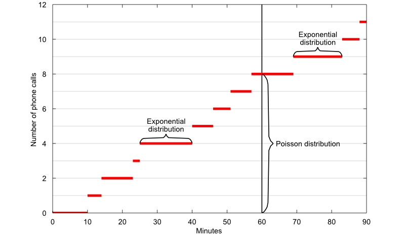
The concept is illustrated by the plot above, where the number of phone calls received is plotted as a function of time. The graph of the function makes an upward jump each time a phone call arrives. The time elapsed between two successive phone calls is equal to the length of each horizontal segment and it has an exponential distribution. The number of calls received in 60 minutes is equal to the length of the segment highlighted by the vertical curly brace and it has a Poisson distribution.
The Poisson distribution deals with the number of occurrences in a fixed period of time, and the exponential distribution deals with the time between occurrences of successive events as time flows by continuously.
The Tweedie distribution is a special case of an exponential distribution.
The probability density function cannot be evaluated directly. Instead special algorithms must be created to calculate the density.
This family of distributions has the following characteristics:
- a mean of $E(Y) = μ$
- a variance of $Var(Y) = φ μp$.
The $p$ in the variance function is an additional shape parameter for the distribution. $p$ is sometimes written in terms of the shape parameter $α: p = (α – 2) / (α -1)$
Some familiar distributions are special cases of the Tweedie distribution:
- $p = 0$ : Normal distribution
- $p = 1$: Poisson distribution
- $1 < p < 2$: Compound Poisson/gamma distribution
- $p = 2$ gamma distribution
- $2 < p$ < 3 Positive stable distributions
- $p = 3$: Inverse Gaussian distribution / Wald distribution
- $p > 3$: Positive stable distributions
- $p = ∞$ Extreme stable distributions
Some Applications:
- modeling claims in the insurance industry
- medical/genomic testing
- anywhere else there is a mixture of zeros and non-negative data points.
try:
    import tweedie as tw
except ImportError:
    !pip install tweedie
    import tweedie as tw
x = np.random.gamma(1e3,size=100) * np.random.binomial(1,p=.3,size=100)
plt.hist(x)
plt.title('Original Population');

mu = x.mean()
sigma = x.std()
mu,sigma
random_tweedie_poisson = tw.tweedie(p=1.01,mu=mu,phi=sigma).rvs(100)
random_tweedie_compound = tw.tweedie(p=1.2,mu=mu,phi=sigma).rvs(100)
random_tweedie_gamma = tw.tweedie(p=1.79,mu=mu,phi=sigma).rvs(100)
random_tweedie_poisson.mean()
random_tweedie_compound.mean()
random_tweedie_gamma.mean()
plt.hist(x,label='Original Population',alpha=.7);
plt.hist(random_tweedie_poisson,label='Random Samples with Tweedie Poisson',alpha=.7);
plt.hist(random_tweedie_compound,label='Random Samples with Tweedie Compund',alpha=.7);
plt.hist(random_tweedie_gamma,label='Random Samples with Tweedie Gamma',alpha=.7);
plt.xlabel('Value')
plt.ylabel('Frequency');
plt.legend(bbox_to_anchor=(1, -0.128),ncol=1);


| VARIABLE NAME | DEFINITION | THEORETICAL EFFECT |
|---|---|---|
| INDEX | Identification Variable (do not use) | None |
| TARGET FLAG | Was Car in a crash? 1=YES 0=NO | None |
| TARGET AMT | If car was in a crash, what was the cost | None |
| AGE | Age of Driver | Very young people tend to be risky. Maybe very old people also. |
| BLUEBOOK | Value of Vehicle | Unknown effect on probability of collision, but probably effect the payout if there is a crash |
| CAR AGE | Vehicle Age | Unknown effect on probability of collision, but probably effect the payout if there is a crash |
| CAR TYPE | Type of Car | Unknown effect on probability of collision, but probably effect the payout if there is a crash |
| CAR USE | Vehicle Use | Commercial vehicles are driven more, so might increase probability of collision |
| CLM FREQ | # Claims (Past 5 Years) | The more claims you filed in the past, the more you are likely to file in the future |
| EDUCATION | Max Education Level | Unknown effect, but in theory more educated people tend to drive more safely |
| HOMEKIDS | # Children at Home | Unknown effect |
| HOME VAL | Home Value | In theory, home owners tend to drive more responsibly |
| INCOME | Income | In theory, rich people tend to get into fewer crashes |
| JOB | Job Category | In theory, white collar jobs tend to be safer |
| KIDSDRIV | # Driving Children | When teenagers drive your car, you are more likely to get into crashes |
| MSTATUS | Marital Status | In theory, married people drive more safely |
| MVR PTS | Motor Vehicle Record Points | If you get lots of traffic tickets, you tend to get into more crashes |
| OLDCLAIM | Total Claims (Past 5 Years) | If your total payout over the past five years was high, this suggests future payouts will be high |
| PARENT1 | Single Parent | Unknown effect |
| RED CAR | A Red Car | Urban legend says that red cars (especially red sports cars) are more risky. Is that true? |
| REVOKED | License Revoked (Past 7 Years) | If your license was revoked in the past 7 years, you probably are a more risky driver. |
| SEX | Gender | Urban legend says that women have less crashes then men. Is that true? |
| TIF | Time in Force | People who have been customers for a long time are usually more safe. |
| TRAVTIME | Distance to Work | Long drives to work usually suggest greater risk |
| URBANICITY | Home/Work Area | Unknown |
| YOJ | Years on Job | People who stay at a job for a long time are usually more safe |
Load Data and Clean Data
df = pd.read_csv('/content/drive/MyDrive/Datasets/car_insurance_claim.csv')

# make columns lowercase
df.columns = df.columns.str.lower()

# drop useless columns
df = df.drop(['kidsdriv','parent1','revoked','mvr_pts','travtime','id','birth'],axis=1)

# clean money amounts
df[['home_val','bluebook','oldclaim','clm_amt','income']] = df[['home_val','bluebook','oldclaim','clm_amt','income']].apply(lambda x: x.str.replace('$','').str.replace(',','')).astype(float)

# clean values from columns
to_clean = ['education','occupation','mstatus','gender','car_type']
for col in to_clean:
    df[col] = df[col].str.replace('z_','').str.replace('<','')

df['urbanicity'] = df['urbanicity'].str.split('/ ',expand=True)[1]

to_clean = ['mstatus','red_car']
for col in to_clean:
    df[col] = df[col].str.lower().replace({ 'yes': True, 'no': False}).astype(int)

df = df.drop(['car_age','occupation','home_val','income','yoj'],axis=1).dropna()

df[:3]
Select Features and Targets
features = ['age','gender','car_type','red_car','tif','education','car_use','bluebook','oldclaim','urbanicity']
binary_target = 'claim_flag'
severity_target = 'clm_amt'
frequency_target = 'clm_freq'
Modeling imports
import xgboost as xgb
import patsy
from sklearn.model_selection import train_test_split
from sklearn import metrics
def clean_col_names(df):
    df.columns = df.columns.str.replace('[T.','_',regex=False).str.replace(']','',regex=False).str.replace(' ','_',regex=False).str.lower()
    return df
Train test split data
train, test = train_test_split(df,random_state=42, test_size=0.33,stratify=df[binary_target])
# select only claims
train_sev = train.loc[train[severity_target].gt(0)]
# create design matrix
pats = lambda data: patsy.dmatrix('+'.join(data.columns.tolist()),data,return_type='dataframe')

# apply design matrix
train_mx = pats(train[features])
train_mx_sev = patsy.build_design_matrices([train_mx.design_info],train_sev,return_type='dataframe')[0]
test_mx = patsy.build_design_matrices([train_mx.design_info],test,return_type='dataframe')[0]

# clean columns
train_mx = clean_col_names(train_mx)
train_mx_sev = clean_col_names(train_mx_sev)
test_mx = clean_col_names(test_mx)
Tree based XGBoost Models
binary_model = xgb.XGBClassifier(objective='binary:logistic', eval_metric='auc', n_estimators=100, use_label_encoder=False).fit(train_mx, train[binary_target])
# gamma model
severity_model = xgb.XGBRegressor(objective='reg:gamma', eval_metric='gamma-nloglik', n_estimators=100).fit(train_mx_sev, train_sev[severity_target])
# poisson model
frequency_model = xgb.XGBRegressor(objective='count:poisson', eval_metric='poisson-nloglik', n_estimators=100).fit(train_mx_sev, train_sev[frequency_target])
Calculate expected Claims
expected_claims = (severity_model.predict(test_mx) * frequency_model.predict(test_mx)) * binary_model.predict_proba(test_mx)[:,1]
var_power = 1.5
tweedie_model = xgb.XGBRegressor(objective='reg:tweedie', eval_metric=f'tweedie-nloglik@{var_power}', n_estimators=100, tweedie_variance_power=var_power).fit(train_mx, train[severity_target])
tweedie_preds = tweedie_model.predict(test_mx)
def lorenz_curve(y_true, y_pred, exposure):
    y_true, y_pred = np.asarray(y_true), np.asarray(y_pred)
    exposure = np.asarray(exposure)
    # order samples by increasing predicted risk:
    ranking = np.argsort(y_pred)
    ranked_exposure = exposure[ranking]
    ranked_pure_premium = y_true[ranking]
    cumulated_claim_amount = np.cumsum(ranked_pure_premium * ranked_exposure)
    cumulated_claim_amount /= cumulated_claim_amount[-1]
    cumulated_samples = np.linspace(0, 1, len(cumulated_claim_amount))
    return cumulated_samples, cumulated_claim_amount

fig, ax = plt.subplots(1,2,figsize=(10, 5))
for label, y_pred in [("Frequency-Severity Model", expected_claims),
                      ("Tweedie Model", tweedie_preds)]:
    ordered_samples, cum_claims = lorenz_curve(test[severity_target], y_pred, test[severity_target].index)
    gini = 1 - 2 * metrics.auc(ordered_samples, cum_claims)
    ax.ravel()[0].plot(ordered_samples, cum_claims, linestyle="-", label=label + " (Gini index: {:.3f})".format(gini))

ordered_samples, cum_claims = lorenz_curve(test[severity_target], test[severity_target], test[severity_target].index)
gini = 1 - 2 * metrics.auc(ordered_samples, cum_claims)
ax.ravel()[0].plot(ordered_samples, cum_claims, linestyle="-.", color="gray",label="Actual (Gini index: {:.3f})".format(gini))

ax.ravel()[0].plot([0, 1], [0, 1], linestyle="--", color="black")
ax.ravel()[0].set(title="Lorenz Curves",xlabel=('Fraction of policyholders\n''(ordered by index of test dataframe)'),ylabel='Fraction of total claim amount')
ax.ravel()[0].legend(loc="upper left")

ax.ravel()[1].hist(test[severity_target],label='Actual Claims')
ax.ravel()[1].hist(expected_claims,label='Frequency-Severity Model')
ax.ravel()[1].hist(tweedie_preds,label='Tweedie Model')
ax.ravel()[1].legend();
ax.ravel()[1].set_title('Claims Distribution');
ax.ravel()[1].set_xlabel('Claim Amount');
ax.ravel()[1].set_ylabel('Frequency');

plt.tight_layout();

The Gini coefficient measures the inequality among values of a frequency distribution (for example, levels of income). A Gini coefficient of zero expresses perfect equality, where all values are the same (for example, where everyone has the same income). A Gini coefficient of one (or 100%) expresses maximal inequality among values (e.g., for a large number of people where only one person has all the income or consumption and all others have none, the Gini coefficient will be nearly one).
With the right parameters calculated from a variable we can use the probability distributions functions to draw samples from the same distribution
- Is important to know how and when to use each distribution when needed based on the target variable and the problem requirements
To aproximate the real distribution you need to draw a large number of samples (kind of obvious but good to have it written down)
Frequency - Severity Model:
- Pros:
- Ability to improve and analyze models individually
- Extend more frequency based models while keeping severity simple
- Ability to improve and analyze models individually
- Cons:
- Highly increased complexity for hyperparameters tunning and feature selection
- Pros:
Tweedie Model:
- Pros:
- Easier to apply tuning techniques for hyperparameters and feature selection since is just one model
- Cons:
- Even though we can choose the ratio between Poisson - Gamma might be hard to maximize the performance from each component of the compound model
- Pros:
We do not have a good metric to meassure how good are our models in solving the insurance expected loss prediction other than the lorezn curve
- can we use PDF to infer the distribution of a variable ?